In the world of trading, one of the greatest challenges is determining future price ranges with enough accuracy to structure profitable trades. One method traders can leverage to enhance these predictions is Monte Carlo simulations, a powerful statistical tool that allows for the projection of a stock or ETF's future price distribution based on historical data.
In this article, I'll introduce Monte Carlo simulations, explain their relevance in trading, and describe a specific options trading strategy I've developed using these simulations. I'll also share backtested results to illustrate the strategy's effectiveness.
1. What Are Monte Carlo Simulations?
Monte Carlo simulations are a computational technique used to model the probability of different outcomes in a process that cannot easily be predicted due to the presence of random variables. Named after the famed casino, these simulations are especially useful in finance because they allow for the analysis of uncertainty and risk.
The process involves running thousands or even millions of simulations based on historical price movements, where each simulation projects a possible future outcome. The resulting distribution provides traders with probabilities of price ranges over a given time horizon.
2. How Are Monte Carlo Simulations Applied in Trading?
In trading, Monte Carlo simulations help to anticipate how a financial instrument, such as an ETF like SPY or QQQ, might behave over a future period. The process looks back over several years of historical price data and runs numerous simulations to project future price distributions. The outputs typically show a probability distribution of future prices, highlighting key metrics such as confidence intervals.Here is an example for SPY:
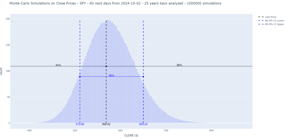
These simulations are invaluable for traders because they offer insights into the probability that a stock or ETF will remain within above/below price bounds over a specific time frame. This information helps to craft structured options strategies, like Credit Put Spreads in Options Trading, which profit when an asset stays above a price threshold.
3. Example for a Credit Put Spread in Options Trading
Here for example is the result of 10,000 simulations carried out on SPY for a prediction of the movement in 15 days by asking the algorithm to calculate what percentage of data is above the $565 threshold. For example if we consider that this value is a support or that this value would be the break even of a Credit Put Spread strategy that we would have implemented.
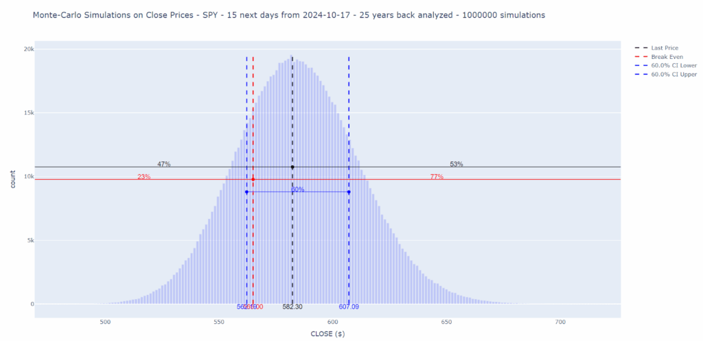
We see that there is a probability of 77% that the ticker is above this threshold value.
Recall that Monte Carlo simulations observe the past behavior of the ticker over many years, day after day, deduce a statistical distribution and perform random shots oriented like this statistical distribution in order to capture the pseudo-random nature of the market. It will be necessary to see how these predictions have come true in the past.
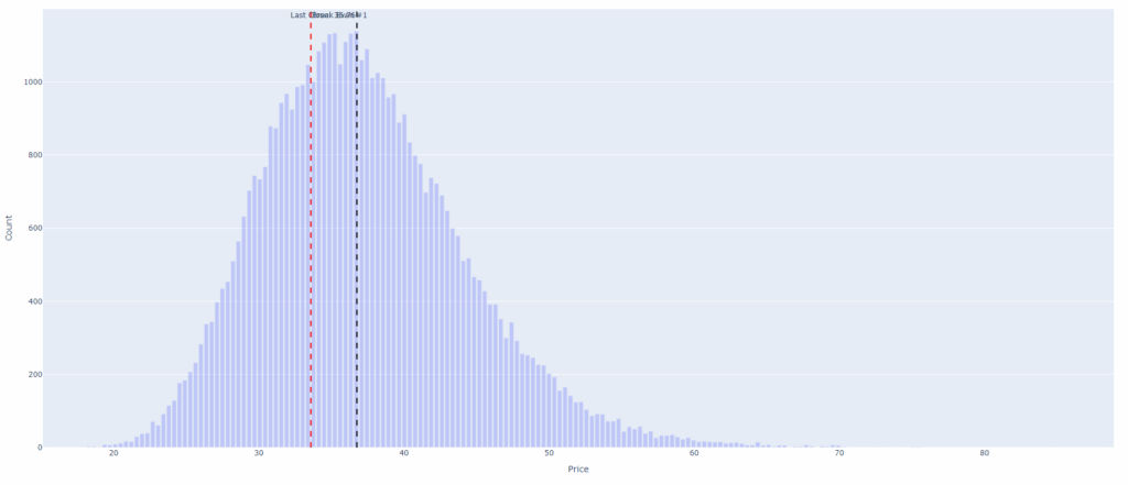
Note that to account for the historical distribution of a ticker, we need to adjust the Monte Carlo simulation approach in the code. Rather than assuming a normal distribution for price movements, I model price changes based on the actual historical distribution of returns. This technique, often called bootstrapping, samples historical returns directly instead of generating synthetic returns based on a fixed normal distribution.
This is then the kind of plot we get :
4. How does the backtesting work?
To address this, I wrote a script that performs the following:
- Go back 15 years in historical data.
- Each day, for 50 of the most liquid tickers in options, perform Monte Carlo simulations using the past 10 years of historical data to determine the ticker's value at which 70%, 75%, 80%, and 85% of the data would be above that value within the next 30, 60, and 90 days.
- Check if, 30, 60, and 90 days later, the ticker's actual price exceeded the threshold value in 70%, 75%, 80%, and 85% of the data. If so, it is a success for Monte-Carlo (score = 1) as it succeeded in forecasting, at least, the threshold. If not it is a zero.
- Record all results (50 tickers x 3 timeframes x 4 probabilities x 15 years x 252 days = 2,268,000 results)
Example of interpretation: If, on March 24, 2012, the Monte Carlo simulations determined that the threshold above which 75% of the data will fall 30 days later is $X, the program checks whether, 30 days later, at least 75% of the data actually exceeds $X. If this is the case, Monte Carlo was correct in making this prediction. Otherwise, it was wrong. The program then counts all the '1's and '0's and provides a score for each ticker, each probability, each period and every day during 15 years.
Here is an extract of the results of these simulations :
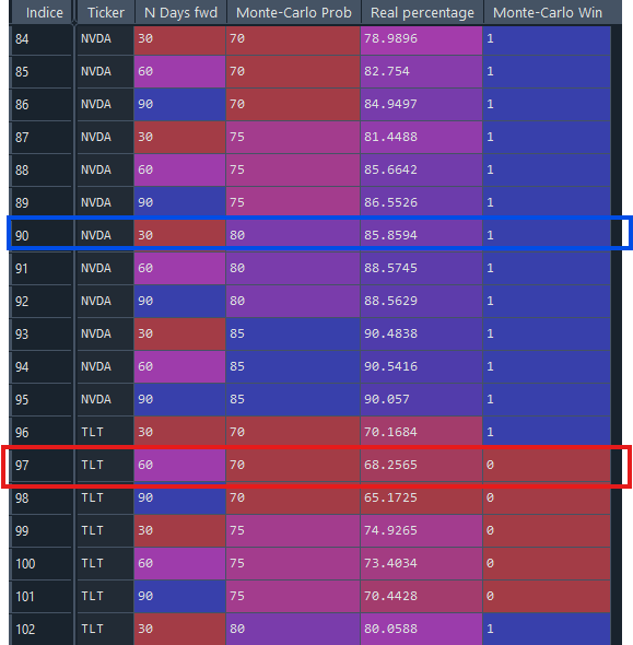
What does it mean?
For the blue rectangle, when Monte-Carlo predicted for 15 years, day after day, that NVDA would be above 80% of a threshold value within 30 days, in reality, it was 85.8594% of the time that the ticker was indeed above the threshold value. So, Monte-Carlo performed better because it underestimated the percentage of times when NVDA would be above a given value (which is good for our potential Credit Put Spread). Therefore, it's a "win" for Monte-Carlo, value "1".
Now, for the red rectangle: when Monte-Carlo predicted that 70% of the data would be above a threshold value within 60 days, it happened 68.2565% of the time. Monte-Carlo overestimated the probability value compared to reality, so it's a "loss", value "0" (but note that the gap between the two percentages is not very high, and therefore the Credit Put Spread is not necessarily at its max loss. We can even imagine it might have been a winner if the algorithm determining the Credit Put Spread was able to find a sufficiently distant breakeven. However, we still count it as a loss).
Finally, the algorithm counts all the 0s and 1s and provides the final result for all the tickers, all the probabilities, and all the periods tested, over 15 years in the past and each time for 2000 Monte-Carlo simulations per day and 10 years of history, in order to determine the distribution law of the Close over the chosen number of days.
For some symbols we even have a 100% win rate (SPY) :
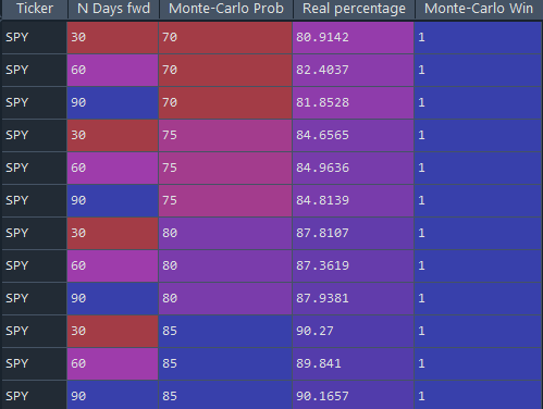
Please note, this does not mean that in 100% of cases, we can predict the prices. It means that, in 100% of cases, when Monte-Carlo says that 75% of the data will be above a given threshold within x days, it is always correct. So, sometimes, x days later, the data will be below the threshold in 25% of cases (and the Credit Put Spread could be a loss).
I believe these results are very encouraging regarding the success rate of Monte Carlo simulations in the past and give us confidence in this type of simulations because, in these backtests, there is no overfitting or bias potential issues : we simply look at the past to see how it would have performed, "purely" — without any fitting or adjustments. It is a straightforward, raw comparison.
Reminder: All analyses derive from historical earnings data and do not account for future surprises or structural shifts. Always combine these insights with forward‑looking research and risk management considerations.